Contents - Previous - Next

Appendix 1: A brief introduction to kinetic studies with tracers

App 1.1: Single pool systems
App 1.2: Systems with two or more pools

Contributor: Andy Coward

App 1.1: Single pool systems

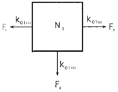
Figure App 1.1 illustrates a single pool of water with volume N and input and output rates equal at a value F per unit time. The fraction of the pool being replaced per unit time is thus F/N and we call this value the rate constant for the system (k).

If a quantity (Q_o) of a tracer is added to this at time zero, calculus shows that:

Q_t = Q_oe^-kt

If N remains constant we can convert this equation for quantity of tracer into one for tracer concentration (C):

C_t =C_oe^-kt

N = pool space
F = flow
k = rate constant where subscript 01 indicates to the outside (O) from compartment 1.

Symbols are as in Figure App 1.1.

Symbols are as in Figure App 1.1.

Thus, the slope of a plot of log C_t against time has the value k and the time zero intercept is C_o. The quantity of tracer added to the system Q_o is the dose given (A) in the context we are discussing here so we can calculate N as A/C_o.

The single pool system we have described has only one exit to the outside. If we consider other exits, as illustrated in Figure App 1.2, it is important to realise that the value k represents the sum of all the fractional losses (k = k₁ + k₂ + k₃) and cannot be used to obtain values for individual exits. These would need to be directly investigated. This leads us to an important concept in analysis of this type, and that is, that the precise nature of the system cannot be deduced unambiguously from tracer data and only if a model is correct will values calculated from tracer data be correct.

App 1.2: Systems with two or more pools

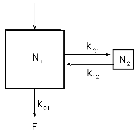
Figure App 1.3 illustrates a simple two compartment system. Let us suppose that N₁ is body-water and N₂ is some other pool with which the ²H or ¹⁸O in water exchanges. In this case if enough observations were made on the isotopic concentration in body-water it would be seen that the disappearance curve consists of two exponential components that add together to produce the observed curve. However, the slopes of these exponentials are not directly equivalent to k₀₁ or any of the other rate constants in the model system. Similarly, the intercepts of the individual exponentials do not directly give the values of N₁, N₂ or (N₁ + N₂) x N₁ is in fact given by the sums of the intercepts.

As far as the present application of the tracer methodology is concerned we have therefore to consider what is likely to happen if a single-compartment solution is applied to a system that is in reality a two-compartment one. For example, in the system in Figure App 1.3 we can assign values of 0.1 and 0.005/day for k₀₁ and k₂₁ respectively and vary k₁₂ from 5 to 0.00005, calculate the characteristics of the curve and then fit a single compartment model to it using early concentration values from Days 0 to 14. With this sampling regime there would be no convincing evidence that a two compartment system existed. Table App 1.1 shows the results. For rapid recycling of isotope predicted volume (N₁) and rate constant (k₀₁) are close to true values and inversely related so that little error is incurred in the measurement of flow (F) as the product (k₀₁)(N₁). However, as the degree of recycling becomes smaller errors in k₀₁ increase because we reach the stage when the estimate of N₁ is correct (recycling is so slow that N₁ cannot see N₂), but k₀₁ is overestimated by 5% as a consequence of the virtually unrecycled losses as k₂₁. The latter case is what is likely to happen to some extent when ²H is sequestered as fat (see Chapter 7). Elsewhere (Chapter 4) it is suggested that rapid recycling of ²H explains the differences between volumes obtained with ¹⁸O and ²H.

Table App 1.1. Effect of different degrees of isotope recycling in a two-compartment system when a one-compartment solution is used

Assumptions used:

k₀₁ = 0.1
k₂₁ = 0.005
k₁₂ = variable
N₁ = 1
F_True = (k₀₁) (N₁) = 0.1

Contents - Previous - Next