Contents - Previous - Next

Chapter 9: Practical consequences of deviations from the isotope elimination model

9.1 Assumptions and the model
9.2 Systematic changes in isotopic turnover
9.3 Random error in the isotopic enrichment
9.4 Summary of theoretical comparison of methods
9.5 Practical comparisons of the two-point and slope-intercept methods
9.6 Conclusions
9.7 References

Contributors:

Dale Schoeller
Andy Coward

9.1 Assumptions and the model

The model for the doubly-labelled water method described by Lifson ¹, is based on two key assumptions about the behaviour of body water. These are that the amount of body-water is constant and that it turns over at a constant rate. This means that disappearance curves for ²H₂O and H₂¹⁸O added to the system are predicted to be mono-exponential.

Strictly speaking neither of these assumptions is correct for any living organism. Water intake and excretion and carbon dioxide production rates change with time, and such changes will affect the linearity of isotope disappearance curves. It will be obvious that if such deviations from the average value are small and of short duration relative to the total measurement period they can be considered as random physiological noise and will have little effect on our calculations. However it is not entirely inconceivable that such changes could be large both in deviation from average values and in terms of duration. In this case it is possible that our techniques for calculation may not be appropriate and may produce biased results. A further factor to consider is random measurement error in all the parameters that enter the model. Thus, the key question is how much error in carbon dioxide production is introduced by random and systematic deviations when current methods of data reduction are applied.

As has been discussed in Section 4.2 the basic formula for reducing the isotopic data for the calculation of CO₂ production is:

r_CO2 = 0.5 (k_ON_O- k_DN_D)

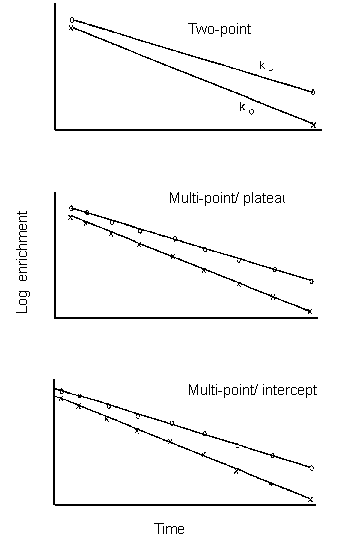
Investigators, however, have chosen three basic aproaches to calculating the elimination rates. They have been calculated using the original two-point method ^1,2 in which the isotopic enrichment is measured at the start and end of the metabolic period, a multi-point method in which the elimination rates are calculated by linear regression of natural log transformed isotopic enrichments ^3,4, or a multi-point method in which elimination rates are calculated from a non-linear curve fit of untransformed data to a mono-exponential equation ⁵ (Figure 9.1). At this meeting two further approaches were suggested, one in which an error structure intermediate between linear and nonlinear regression (i.e. Poisson) is assumed, and a fifth in which the elimination parameters are calculated from a regression analysis of the isotope enrichment products (C_OC_D) and ratios (C_O/C_D) (see Chapter 5). This method, however, leads to the identical CO₂ production rate as the single isotope fits and only the estimate of precision is changed because covariance of ²H and ¹⁸O data is taken into account. In addition, each of these methods has two possible variants, one in which a single isotope dilution space is measured and the other space is assumed to be a fixed proportion of the first ² and the second variant in which both isotope dilution spaces are measured ^{3, 4}. For the two-point method, the dilution spaces are typically measured by the plateau method in which the isotopic enrichment is measured at an equilibrium which is assumed to occur two to six hours after the dose. For the multi-point method, the dilution spaces are usually calculated from the zero-time isotope enrichments predicted by the regression line.

Note: In practice all current users of the multi-point version employ variable pool spaces. Comparisons between two-point and multi-point with fixed pools are therefore somewhat unnecessary.

9.2 Systematic changes in isotopic turnover

Two factors could systematically alter isotope turnover rates in doubly-labelled water studies. These are step changes in either carbon dioxide production or water flux. In order to determine how sensitive the doubly-labelled water method is to such systematic variations, a series of synthetic data sets were computer generated.

9.2.1 Methods

The model assumed a typical adult male receiving a loading dose of 0.119 g ²H₂O and 0.247 g H₂¹⁸O (initial isotopic enrichments of 660 and 110 ‰, respectively) and having isotope elimination rates of 0.1050 and 0.1300 d-1 for ²H and ¹⁸O respectively. N_D was 2217.8 moles (401) and N_O was 2153.2 moles (38.31). N_D/N_O was thus 1.03. Daily isotopic enrichments were calculated for these basal conditions and then for 30% increases in CO₂ production and water flux in which sustained increases occurred during Days 1-6, 7-12 or 13-18 of an 18 day measurement period. Isotope dilution spaces and elimination rates were then calculated from the synthetic data and the accuracy of the data reduction method was determined as the percent error relative to the true average CO₂ production rate.

It should be noted that the assumption of a 30% change in carbon dioxide production is rather extreme. For example, a subject with a daily energy expenditure of 1.5 x BMR would have to increase this to 1.95 x BMR. Physical activity would have to increase by 150% in order to achieve this since BMR and obligatory thermogenesis account for a relatively constant 1.15 -1.20 x BMR. The postulated increments in CO₂ production may therefore be regarded as somewhat unphysiological and clearly, if the frequency of the changes is increased, errors will be smaller. This is indicated by the values for 3-day rather than 6-day cycles in Table 9.1.

Table 9.1. Effect of a 30% increase in CO₂ production during one third of a two half-life metabolic period for energy expenditure

¹ Assumes N_D/N_O = constant: (1.03).

² Uses individually calculated values of N_O and N_O.

³ Calculated from initial and final enrichment.

⁴ Calculated from least squares regression of the transformed enrichment.

⁵ Calculated from least squares fit c = c_oe^-kt

9.2.2 Systematic errors due to changes in CO₂ production

Systematic errors in CO₂ production for the three basic data reduction techniques are compared in Table 9.1 for a metabolic period of 18 days. In each case the two-point method shows no error because it provides an exact average when rates vary, if, as assumed here, N_O and N_D are correctly determined from plateau values (see Section 4.4.1). When a fixed pool model is used (ie it is assumed that N_O/N_D is constant) errors for the linear regression technique are only -2 to +4%. In contrast the nonlinear regression method is in error by -6 to +5% with the largest errors occuring when the increase occurs early or late in the metabolic period. This is because the non-linear method heavily weights the early data points and thus the elimination rates reflect the values of the first half of this data rather than the average. It should however be noted that no group using multi-point data employ fixed pool size ratios.

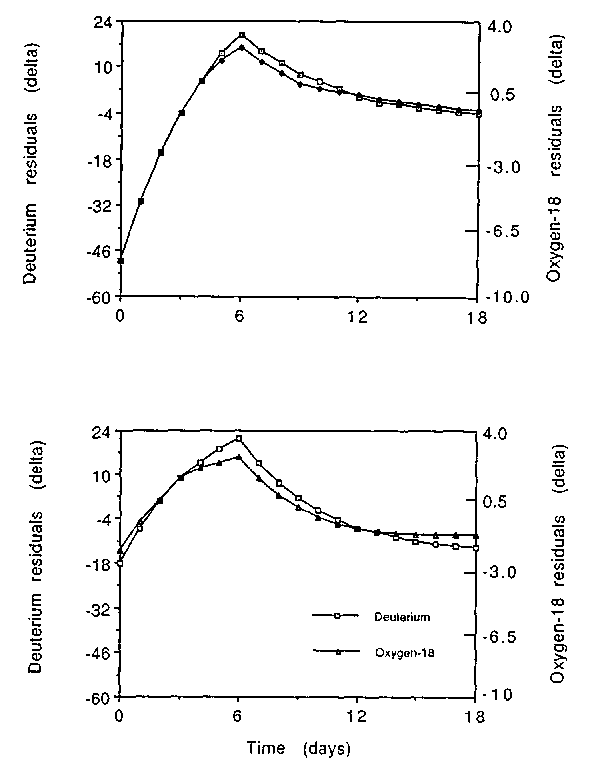
When a variable pool model is used (ie both isotope dilution spaces are calculated) the errors in CO₂ production increase dramatically as both methods show errors in CO₂ production in excess of 5%. This is because the intercepts no longer give the correct values for N_O and N_D. Inspection of residuals of differences between fitted and observed values exposes this problem (see Fig 9.2).

9.2.3 Systematic errors due to changes in water flux

The errors in CO₂ production due to systematic variation in water flux are compared for the three basic methods of data reduction in Table 9.2. As was observed for increases in CO₂ production, the two-point method always gives the exact average and hence zero systematic error if N_O and N_D are correctly estimated. Similarly if N_O and N_D are correctly measured from an isotope plateau, the linear regression method was also very robust as errors are less than 1%. The non-linear regression method, however, is still subject to large systematic errors of up to 6%.

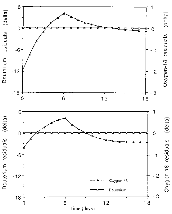
When the variable pool model is used and both isotopic dilution spaces are calculated by back extrapolation to zero time, the systematic errors again increase for the linear regression method. This is due to a systematic difference between the intercept calculated from the regression line and the true zero-time value that is evident from the early elimination data as evident from the residual plots (Figure 9.3). There is, however, little effect on the non-linear regression method, because it heavily weights the early data and thus leads to smaller residuals and hence error in the intercept.

In common with systematic increases in CO₂ production, there is very little error if the increased water flux occurs at regular intervals throughout the metabolic period.

This analysis identifies potential pitfalls associated with multi-point methodology. The discrepancies do not arise from an error in the method, but instead are an example of the wrong answer being generated by using a procedure in circumstances for which it was not designed. It should be noted that either the propagation of error analysis suggested in Chapter 5 or a simple residual plot of the multi-point data would quickly identify a data-set suffering from such a discontinuity. It should then be rejected or recalculated by the two-point method if the sampling protocol included collection of 'plateau' post-dose samples.

Upper panel - Linear regression
Lower panel - Non-linear regression

Upper panel - Linear regression
Lower panel - Non-linear regression

Table 9.2. Effect of a 30% increase in water turnover during one third of a two half-life metabolic period for energy expenditure

Superscripts as in Table 9.1.

9.3 Random error in the isotopic enrichment

Each of the data reduction techniques differs in robustness with regard to the effect of random error in isotopic enrichment which occurs during sample collection, treatment and isotopic analysis. This question of random analytical error is especially critical for the first time user of doubly-labelled water because high precision isotopic measurements are quite demanding. As indicated in other chapters, the isotopic enrichments are small with regard to the absolute amount of excess isotope and analytical errors that result from isotope fractionation during sample handling and analysis can be significant relative to the actual enrichment. This introduces an error in the calculated CO₂ production and reduces the precision of the technique.

9.3.1 Methods

Random error was added to the initial data set and the CO₂ production rate calculated using the same data reduction methods as in the above section on systematic error. Each data set included fifteen decay curves with random error which were then subjected to the three modes of data reduction. The precision of the doubly-labelled water method with regard to CO₂ production was calculated from the standard deviation about the mean. This was expressed as the percent of total CO₂ production. Random error was added to the isotopic enrichment at each time point using a computer program that assigns error randomly based on the normal Gaussian distribution. To do this, we assumed a random error level from literature ⁶ in which the 18o analytical error was 0.18 ‰ at zero enrichment and increased linearly to 0.97 ‰ at an enrichment of 260 ‰ The analytical error for the deuterium was taken to be 1.2 ‰ at zero enrichment and increased linearly to 3.2 ‰ at an enrichment of 590 ‰.

In addition, the effects of a high analytical error were investigated assuming random errors equal to 3 times the above errors. Two error analyses were performed. In the first analysis, it was assumed that there was no error in the baseline measurement and that all the error was contained in the enrichment data. In the second analysis it was assumed that error was present in the baseline and the sample. Thus, the enrichment data for each data-set contained a baseline error or offset and random error in each time point.

The effect of random errors in the two-point method of calculating CO₂ production were initially discussed by Lifson ⁷ and Nagy ⁸. This has been extended by Schoeller ⁹. In these discussions, it was generally observed that the best precision of the doubly-labelled water method occurs between one and three biological half-lives of the isotopes. For shorter metabolic periods, the isotopic change is small relative to analytical error and precisions of less than 5% are hard to obtain at economical isotopic doses. For longer metabolic periods, the final isotopic enrichment is small relative to the analytical error and precisions of less than 5 to 10% are hard to obtain. The sensitivity to analytical error was therefore calculated for metabolic periods of 2 biological half-lives.

9.3.2 Effect of random error on the precision of calculated CO₂ production

The effect of random error in the enrichment data is summarised in Table 9.3. In contrast to the previous systematic physiologic effects, the multi-point methods were more robust in the face of random error than the two-point method by a factor of between 1.5 and 2. At the lower levels of analytical error, however, all three methods provided precisions of 5% or better. When the variable pool method was used and the two isotopic dilution spaces were calculated from the enrichment data, there was a 39% improvement in the precision of the multi-point methods. This improvement illustrates the effect of the negative covariance of the slope and intercept of a regression line in the presence of random error (see Chapter 5).

When the large analytical error was applied, the precision of the two-point method was very poor (Table 9.3 and Figure 9.4), and is not improved by using the two calculated dilution spaces. The precision of the linear regression technique was also poor, but was improved when intercept data rather than plateau data was used for volume determinations. The extent of the improvement (35%) was about the same as that observed in the case of moderate analytical error.

When the effect of baseline random error is added to the analysis, precision for all methods worsens (Table 9.4). With the large analytical error, the precision of the two-point method is quite poor and would be unacceptable for almost all applications. The multi-point method performs much better, but precisions are still worse than 8% and thus unacceptable for many applications of the method. In general, the non-linear regression technique provided better precision than the linear regression method because it weighted the average in favour of the earlier time points that had a smaller relative error.

Contents - Previous - Next