In this section the ten Cambridge workshop datasets are used as examples to illustrate the precision and accuracy of estimated CO2 production.
The standard error of r'CO2 calculated from Equation 13 ranges from 0.7% to 4.0% over the ten datasets, with a median of 1.6%. The bias for each dataset is obtained from the residual for the first sample after 5 hours on the 'product' line, halving it and changing its sign. The bias from the 'ratio' plot is assumed here to be zero, since all the NO/ND ratios are reasonable in value. The 'product' bias over the ten datasets has a mean of 0.1% and a standard deviation of 2.1%. Thus the standard deviation for precision is 1.6% and for accuracy it is 2.1%. These two errors are independent, so they can be combined as their root mean square. This gives a combined error of 2.6%. The overall mean bias of 0.1% is trivially small. It should be noted that the Cambridge datasets were selected from sequential analyses from a large database, and were not selected as being particularly well-behaved data.
It is instructive to repeat this exercise for the two-point method. Here there is no bias, so the error is all in the precision. Normally it is not possible to calculate the precision as there are no degrees of freedom for error. However an estimate of the precision can be obtained by assuming that the errors around the 'product' and 'ratio' lines in the multi-point method, sp and sr in Equation 13 are the same as in the two-point method. On this basis the terms involving s, A and B in Equation 13 are unchanged, but n is reduced to 2, and St² is calculated from just the first and last points of each dataset. This then provides an estimate of the variance of r'CO2 which can be compared with the multi-point method.
Doing this sum for the Cambridge
datasets shows that the precision variance is increased by a median factor of 5.0 (range
4.2 to 5.9), giving a median error of ![]() ,
where 1.6% is the multi-point precision. Thus the multi-point method has a combined
precision and accuracy of 2.6%, whereas for the two-point method the figure is 3.6%.
,
where 1.6% is the multi-point precision. Thus the multi-point method has a combined
precision and accuracy of 2.6%, whereas for the two-point method the figure is 3.6%.
The log regression analysis assumes that the error about the regression line does not change systematically with the level of enrichment (ie the absolute error is proportional to the enrichment). In theory (Section 9.3) physiological error should satisfy this assumption quite well, whereas analytical error tends to be relatively smaller at high enrichments. So, depending on the relative magnitude of the two sources of error, enrichment error should lie somewhere between constancy and proportionality. Although the analytical error varies from laboratory to laboratory, it should be much smaller than the physiological error unless enrichments are small, so that the assumption of proportional errors is usually reasonable on average over a large number of subjects. Some individuals may exhibit error structures which deviate from this model (see for example James et al ²) largely because of temporal variability in water intake.
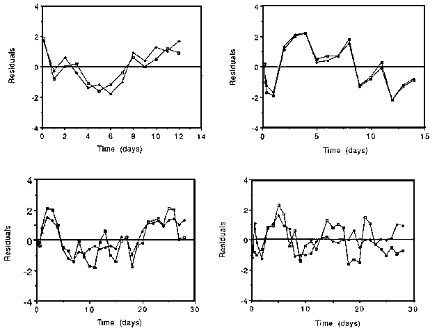
When there is evidence that the errors are nearer to constant than proportional, an absolute form of analysis can be used which fits an exponential curve to the absolute enrichments. This approach may suit the analytical error structure, but it is usually inappropriate for the physiological error, which being relatively constant gets smaller in absolute terms as the enrichment falls. As a result the exponential fit concentrates on the large errors at the start of the experiment and pays little attention to the later data (see also Section 9.2.2). Figure 5.2 illustrates residuals from 4 data-sets which show equally large residuals at the end of the experiment as at the beginning, and for which use of an exponential fit may therefore be preferable.
There is an intermediate form of analysis which assumes Poisson type errors, where the errors increase as the square root of the enrichment. This can be viewed as a compromise analysis, to be used when the error structure is neither constant nor proportional. It is possible to compare the effects of the three approaches in an approximate way by using weighted log regression, where the individual points are given weightings as follows:
a) for errors proportional to enrichment, use weighting = 1
b) for constant errors, use weighting = enrichment ²
c) for in-between errors, use weighting = enrichment.
If the results change substantially using the different weighting systems, this suggests a pathological pattern of residuals which inspection of the residual plots (see Section 5.10) should clarify. (Note that the weighted regressions (b) and (c) require, in theory, an iterative procedure for the true weightings are unknown, but in practice use of the observed enrichments usually suffices.)
Note: The units (ppm normalised to 100 at zero time) differ from those used in Chapter 11.
It is probable that the unweighted
log regression (equivalent to (a) above) is the most useful analysis, as it is easy to do
even on a hand calculator, and it fits in with the ratio and product plot procedures
described earlier.
The production of diagnostic plots is an important stage in the fitting process. There are two useful forms of plot, data plots and residual plots. In general the values for 18O and 2H can be plotted on the same graph, while the product and ratio data need to be treated separately.
Each data plot indicates the observed enrichments, on a log scale, plotted against time, with the fitted linear regression line superimposed. The residual plot shows the residuals from each enrichment (ie the observed values less the value predicted from the fitted line) plotted against time. In general, the residual plots show whether or not the assumption of a constant proportional error variance is valid. If the magnitude of the residuals appears to increase systematically with time then this is evidence against, and one of the alternative analyses discussed in Section 5.9 may be considered more suitable.
The natural log scale on the Y axis of the residual plot can be rendered more comprehensible by multiplying it by 100, and calling it a percentage scale. This is highly accurate for log values up to +/- 0.1, ie +/- 10%, but becomes progressively less accurate for higher values. Thus a residual of -0.06 indicates that the observed enrichment is 6% less than the enrichment predicted by the regression line at that time.
There are other features to look for in each type of plot, which are dealt with separately.
5.10.1 18O and 2H plots
It is important that the results for the two isotopes should be plotted on the same graph - they then show the degree of covariance between 18O and 2H. Both data and residual plots also give a measure of the size of the errors, evidence for any systematic departures from linearity, and evidence for errors increasing or decreasing through the experiment.
5.10.2 Product plot
The most important part of the product data plot is the intercept of its regression line, as this estimates the zero time enrichment and hence the body water pool size. The product plot often shows signs of serial correlation (also known as auto-correlation), where the residuals at particular time points are similar to the residuals near them in time. Put another way, it means that the data follow a curve which differs systematically from a straight line. The product plot is better than the 18O and 2H plots for seeing signs of this non-linearity, as the two trends are combined.
If there is evidence of serial correlation then the intercept is likely to be a biased estimate of the zero time enrichment (see Section 5.7), and the magnitude of this bias can be read off the residual product plot. However it is important to remember to halve the value so obtained, as it is the sum of the biases for the two isotopes. The CO2 production rate is then biased to this extent in the opposite direction, as the intercept is the inverse of the pool size.
It is possible to test formally for the presence of curvature in the product plot, but in practice it is more important to read off the likely bias of the intercept from the residual plot.
5.10.3 Ratio plot
The ratio plot is a very sensitive way of presenting information about the CO2 production rate, and as such is useful for assessing the linearity of the plot and constancy of production. In addition, the intercept of the ratio data plot is the log of the ND/NO ratio, and should normally be about +0.03, corresponding to a ratio of 1.03. Since the plot declines with time, the fitted line normally crosses the time axis during Day 2. If there are several residuals during the first day, and if they are all systematically non-zero, then this may indicate bias in the ND/No ratio. Section 5.7 shows how this bias translates to a five-fold bias in the CO2 production rate.
Worked examples illustrating many of
the points raised here are presented in Chapter 11.
1. Coward WA, Roberts SB & Cole TJ (1988) Theoretical and practical considerations in the doubly-labelled water (2H218O) method for the measurement of carbon dioxide production rate in man. Eur J Clin Nutr; 42: 207-212.
2. James WPT, Haggarty P & McGaw
BA (1988) Recent progress in studies on energy expenditure: are the new methods providing
answers to old questions? Proc Nutr Soc; 47: 195-208.